
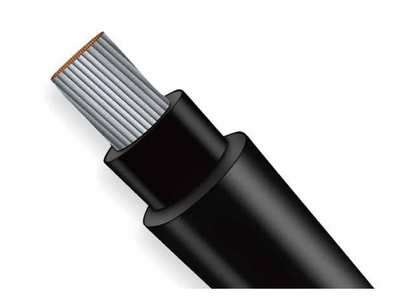
Moving from 4 mm² to 6 mm² solar cable reduces conductor resistance and therefore voltage drop and cable heating at the same current and route length. Whether that improvement is worthwhile depends on the PV string operating voltage, actual cable route and installed current rating. In the worked example below—a 50 m one-way route carrying 20 A—the calculated drop falls from 10.18 V to 6.78 V using reference conductor resistances at 20°C. Those figures compare two cable sizes; they do not establish the maximum safe current or an approved string design.
Place the cable size on the correct circuit first
A commercial rooftop or ground-mounted PV plant can contain many individual string circuits. A pair of 4 mm² or 6 mm² conductors may carry one string to its DC collection or conversion equipment. After strings combine, the current in the shared circuit changes. That shared cable needs its own sizing calculation.
Module strings connected in series add voltage, while parallel strings add current. A cable decision based only on total inverter kilowatts can therefore miss the circuit actually served by the conductor.
The size marking describes nominal conductor cross-sectional area, not the outside diameter of the cable. XWA’s H1Z2Z2-K solcellekabel is a product route for PV DC wiring; the selected construction, voltage rating and connector arrangement remain part of the cable schedule.

EN 50 m route includes 100 m of conductor
For a simple two-conductor DC circuit, current travels through the positive conductor and returns through the negative conductor. If each follows the same 50 m route, the resistance calculation includes 100 m in total. Any additional module leads or extensions contribute their own resistance.
Calculation basis: 20 A operating current; 50 m one-way length; equal positive and negative cable sizes; ledermodstand ved 20°C. The example uses 5.09 Ω/km for 4 mm² og 3.39 Ω/km for 6 mm² from the selected tinned-copper reference cable schedule. Connector resistance and other circuit sections are excluded.
Loop resistance (Ω) = 2 × one-way length (m) × conductor resistance (Ω/km) ÷ 1000
Voltage drop (V) = operating current (EN) × loop resistance (Ω)
Cable loss (W) = operating current² × loop resistance (Ω)
| På 20 A and 50 m one-way | 4 mm² cable | 6 mm² cable |
|---|---|---|
| Conductor resistance at 20°C | 5.09 Ω/km | 3.39 Ω/km |
| Positive + negative length | 100 m | 100 m |
| Calculated loop resistance | 0.509 Ω | 0.339 Ω |
| Calculated voltage drop | 10.18 V | 6.78 V |
| Drop relative to 600 V operating voltage | 1.70% | 1.13% |
| Instantaneous loss in this cable pair | 203.6 W | 135.6 W |
For this defined case, 6 mm² reduces the calculated cable-pair loss by 68 W, approximately one third. That is an instantaneous comparison at the assumed current and resistance, not an annual energy-yield prediction. Irradiance, current and cable temperature change during operation.
Change the operating voltage, and the percentage changes
If the same 20 A and cable resistance were compared against a 1000 V operating voltage instead of 600 V, the drop would still be 10.18 V or 6.78 V. The percentages would become approximately 1.02% og 0.68%. The conductor has not improved; the voltage used as the percentage reference has changed.
Use the string operating voltage for the operating-loss comparison. Cold-condition open-circuit voltage serves a different check: it must remain within the applicable cable, equipment and system voltage limits. A lower percentage at a higher operating voltage is not permission to add modules to a string without that separate design check.
A project voltage-drop target also needs a defined boundary. A target for one home-run cable pair differs from a target for the complete DC path including module leads, collection circuits and connections. The number becomes useful when its circuit boundary and operating case are stated.
Current capacity is a separate calculation
De 20 A example illustrates resistance and loss. Installed ampacity depends on conductor temperature limits, omgivende forhold, grouping, enclosure and routing. Design current and protective-device coordination must also reflect the PV array configuration and applicable installation rules.
Resistance increases as copper becomes hotter, so a calculation using 20°C resistance can understate operating drop on a hot route. For a final design, use resistance at the relevant conductor temperature or a documented temperature correction. Ambient air temperature and conductor temperature are different inputs.
IEC 62548-1 treats array wiring alongside electrical protection, switching and earthing. IEC 62930 addresses the PV cable itself. Keeping the system design and the cable specification distinct avoids treating a product rating as approval of the whole circuit. Our solar cable standards explanation covers that product-standard context.
The inverter’s AC output is another circuit, with its own current, installation and protection requirements. That feeder belongs with the appropriate low voltage power cable range, rather than inheriting the DC string-cable choice.
The connector and cable entry change with the cable
A larger conductor needs the corresponding contact and crimp range. Its finished outside diameter must also match the connector’s cable seal. Matching the conductor area alone leaves part of the interface unresolved.
Sandia’s connector reliability research examines the consequences of poor installation, mismatching and degraded connections. For en 4 mm²-to-6 mm² change, a matched connector, contact, seal and assembly process are part of the specification—not an accessory decision deferred until installation.
Routing deserves the same attention. Støtte, bend space and protection against abrasion allow the selected cable to perform its intended role. More copper lowers resistance; it does not correct an unsupported cable or a strained connection.
Where we would use the extra copper
For a long string route, we would compare the installed loss and connector arrangement before standardising a cable size. Six square millimetres can be worthwhile where its lower resistance meets a meaningful project loss target. Four square millimetres remains a reasonable option where the current, rute, voltage-drop target and interfaces are all satisfied.
A plant-wide cable schedule can therefore contain both sizes. Shorter string runs and longer home runs need not share one answer merely for purchasing simplicity. The calculation should make the trade-off visible before the installation lengths are committed.
For a PV cable supply discussion with XWA, send the string current, driftsspænding, positive and negative route lengths, quantity and connector details. Those inputs help turn a generic 4 mm²/6 mm² comparison into a cable schedule for the project.